Gradient Descent
One parameter
- Let’s suppose true phenomenon is
y <- 6x• but we don’t know the exact relationship so we assume
y <- ax• using sum of squared errors as the loss function
yhat <- ax1
 residual <- yhat — y
 residual <- ax-y

 residual² <- (ax — y)²• let residual² = loss function()• so lossfunction() <- (ax — y)²
- Only thing we can vary the residuals with is by changing a. x and y are constants given by our dataset.
- Consider the differential below
d lossfunction()
 — — — — — — — — <- 2*(ax-y)
 d a
Lets see how change in a changes residuals
library(ggplot2)
 library(dplyr)
 library(tidyr)
 a <- c(1,2,3,4,5,6,7,8,9,10,11)

 x <- c(8,9,10,11,12,13)
 y <- 6*x + rnorm(length(x) , sd = 1.5) # random noise

 residuals <- sapply(a, function(a) sum((a*x — y)²) )

 ggplot(data = data.frame(coff = a , res = residuals), aes(x = coff , y = res)) +
 geom_point() +
 geom_smooth()
- We expected a parabola because
lossfunction() <- $_ (ax — y)²• We see that the minimum residuals are achieved when coff = 6 which is our true parameter.
• what if we had 2 params
Two Parameters
• Suppose our true relationship is
y = 7*x1 + 2*x2• about which we don’t know so we assume
y = a*x1 + b*x2• we want to find best a and b that describe my data/fit my data well.
• we again use our least square loss function.
residual = (yhat — y)
 = (ax1 + bx2 — y)

 residual² = (ax1 + bx2 — y)²
• what we can change here are both a and b.
so d lossfunction() — — — — — — — = 2x1(ax1 + bx2 — y) d aso d lossfunction() — — — — — — = 2x2(ax1 + bx2 — y) d b
But now its difficult for us to visualize since there are 3 dimensions 1. Total Loss 2. a 3. b
a <- c(4,5,6,7,8,9,10)
 b <- c(-1,0,1,2,3,4,5)

 x1 <- c(8,9,10,11,12,13)
 x2 <- c(100,120,130,140,80,70)


 #since its linear combination we would want to scale all the independent variables

 work <- function(x1 , x2, a,b){

 x1 <- scale(x1)
 x2 <- scale(x2)

 # True
 # y = 7*x1 + 2*x2

 y <- 7*x1 + 2*x2 +rnorm(length(x) , sd = 1.5) # random noise

 ecomb <- expand.grid(a,b) %>% as.data.frame()
 colnames(ecomb) <- c(“a” , “b”)

 ecomb$residuals <- sapply(a, function(a) sapply(b , function(b) sum((a*x1 + b*x2 — y)²))) %>%
 matrix(nrow = length(a)*length(b))

 head(ecomb %>% filter(a == 7 | b == 2))

 gathered <- ecomb %>% gather(key=”coefname” , value=”coefvalue” , -residuals)

 ggplot(data =gathered , aes(x = coefvalue , y = residuals) ) +
 geom_point(width = 0.1) +
 geom_smooth(color = ‘green’) +
 geom_hline(yintercept = 0 , color = ‘blue’) +
 facet_grid(~coefname) +
 geom_vline(data = data.frame(coefname=c(“a” , “b”) , z=c(7.0,2.0)) , aes(xintercept = z) , color = ‘yellow’)
 }

 work(x1 ,x2, a,b)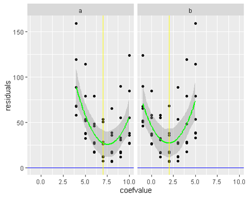
We get slight errors in our a and b estimate but thats due to small sample size. If we increase the sample size to be 100 instead of 7
## Same coef values as above
 a <- c(4,5,6,7,8,9,10)
 b <- c(-1,0,1,2,3,4,5)


 ### Increased Sample Size to 100
 x1 <- rnorm(100 , 10 , 5)
 x2 <- rnorm(100 , 100 , 10)


 work(x1 ,x2, a,b)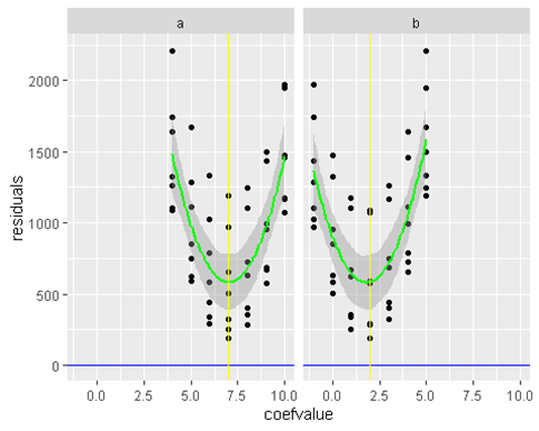
Gradient Descent
• Now the idea is to use a loss function and an algorithm that would find the minima of our loss function. One such algorith is gradient descent.
• The algorithm would travel the green line in our above examples and find the minima and therefore the corresponding values of a and b which are minimizing the loss function (in our case above — Sum of squared errors)
• No matter how many parameters concept remains the same — to find the minima of the loss function
• Lets return the simple 1 parameter example
a <- c(1,2,3,4,5,6,7,8,9,10,11)

 x <- rnorm(100)
 y <- 6*x + rnorm(length(x) , sd = 1.5) # random noise

 residFunc <- function(a) sum((a*x — y)²)

 residuals <- sapply(a, residFunc)

 slope = function(a){ sum(2*x*(a*x — y)) }


 learningRate <- 0.001
 startingA <- 11


 gradiantDescent <- function(startingA, learningRate , iter = 10){
 aestimate <- startingA
 estimates <- c()
 stepStop <- 0.1

 for( i in seq(1,iter,1) ){
 step <- slope(aestimate)*learningRate
 if(abs(step) < stepStop) break
 newAEstimate <- aestimate — step
 aestimate <- newAEstimate
 print(aestimate)
 estimates <- c(estimates , aestimate)
 }
 estimates
 }

 estimates <- gradiantDescent(startingA , learningRate , 20)[1] 10.13894
 [1] 9.421883
 [1] 8.824738
 [1] 8.327455
 [1] 7.913334
 [1] 7.568467
 [1] 7.281272
 [1] 7.042106
 [1] 6.842936
 [1] 6.677074
 [1] 6.538949
 [1] 6.423924
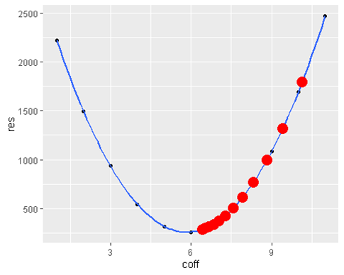
ggplot(data = data.frame(coff = a , res = residuals), aes(x = coff , y = res)) +
 geom_point() +
 geom_smooth() +
 geom_point(data = data.frame(x = estimates , y = sapply(estimates, residFunc )) , aes(x=x, y=y) , color = ‘red’ ,size=5)ggplot(data = data.frame(x = estimates ), aes(y = x , x = seq(1:length(x)))) +
 geom_point() +
 geom_smooth()
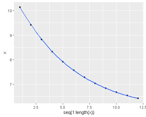
- What if we change our starting a estimate or our learning rate
startingA = 100
learningRate = 0.001
iter = 100
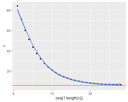
estimates <- gradiantDescent(startingA , learningRate , iter)[1] 84.25529
[1] 71.14359
[1] 60.2246
[1] 51.13161
[1] 43.55926
[1] 37.25325
[1] 32.00181
[1] 27.62857
[1] 23.98669
[1] 20.95384
[1] 18.42818
[1] 16.32489
[1] 14.57334
[1] 13.11471
[1] 11.90001
[1] 10.88844
[1] 10.04604
[1] 9.344515
[1] 8.760308
[1] 8.2738
[1] 7.868652
[1] 7.531257
[1] 7.250285
[1] 7.016301
[1] 6.821447
[1] 6.659178
[1] 6.524046
[1] 6.411513ggplot(data = data.frame(x = estimates ), aes(y = x , x = seq(1:length(x)))) +
geom_point() +
geom_smooth() +
geom_hline(yintercept = 6 , color = ‘red’)
We can see that it converges to the truth of 6
- Lets change the learning rate
startingA = 100
 learningRate = 0.002
 iter = 100

 estimates <- gradiantDescent(startingA , learningRate , iter)[1] 68.51057
 [1] 47.55323
 [1] 33.60537
 [1] 24.32257
 [1] 18.14453
 [1] 14.03283
 [1] 11.29634
 [1] 9.475114
 [1] 8.26302
 [1] 7.456329
 [1] 6.919446
 [1] 6.562132
 [1] 6.324327
 [1] 6.166058
 [1] 6.060725ggplot(data = data.frame(x = estimates ), aes(y = x , x = seq(1:length(x)))) +
 geom_point() +
 geom_smooth() +
 geom_hline(yintercept = 6 , color = ‘red’)
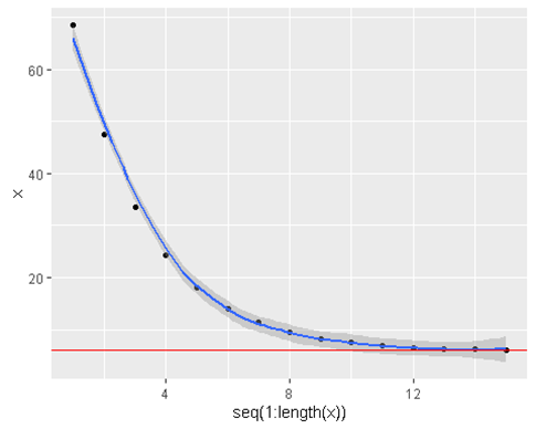
- We see that the algorithm converges much more quickly when we increase the learning rate
• But what if we increase it too much ?
startingA = 100
 learningRate = 0.005
 iter = 100

 estimates <- gradiantDescent(startingA , learningRate , iter)[1] 21.27643
 [1] 8.378402
 [1] 6.265195
 [1] 5.918968ggplot(data = data.frame(x = estimates ), aes(y = x , x = seq(1:length(x)))) +
 geom_point() +
 geom_smooth() +
 geom_hline(yintercept = 6 , color = ‘red’)
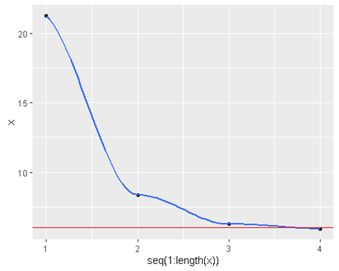
- Converges at an even faster rate
startingA = 100
learningRate = 0.1
iter = 100
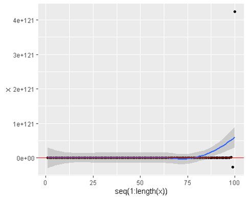
estimates <- gradiantDescent(startingA , learningRate , iter)[1] -1474.471
[1] 23281.27
[1] -365958.5
[1] 5754140
[1] -90473445
[1] 1422533037
[1] -22366785121
[1] 351677652498
[1] -5.529501e+12
[1] 8.694151e+13
[1] -1.367e+15
[1] 2.149362e+16
[1] -3.379487e+17
[1] 5.313639e+18
[1] -8.354745e+19
[1] 1.313634e+21
[1] -2.065454e+22
[1] 3.247557e+23
[1] -5.106203e+24
[1] 8.028589e+25
[1] -1.262352e+27
[1] 1.984822e+28
[1] -3.120778e+29
[1] 4.906865e+30
[1] -7.715166e+31
[1] 1.213072e+33
[1] -1.907338e+34
[1] 2.998948e+35
[1] -4.715308e+36
[1] 7.413978e+37
[1] -1.165715e+39
[1] 1.832879e+40
[1] -2.881874e+41
[1] 4.53123e+42
[1] -7.124548e+43
[1] 1.120208e+45
[1] -1.761326e+46
[1] 2.76937e+47
[1] -4.354338e+48
[1] 6.846417e+49
[1] -1.076477e+51
[1] 1.692567e+52
[1] -2.661258e+53
[1] 4.184352e+54
[1] -6.579144e+55
[1] 1.034453e+57
[1] -1.626492e+58
[1] 2.557367e+59
[1] -4.021001e+60
[1] 6.322305e+61
[1] -9.940692e+62
[1] 1.562996e+64
[1] -2.457531e+65
[1] 3.864028e+66
[1] -6.075492e+67
[1] 9.552624e+68
[1] -1.501979e+70
[1] 2.361593e+71
[1] -3.713182e+72
[1] 5.838315e+73
[1] -9.179704e+74
[1] 1.443344e+76
[1] -2.2694e+77
[1] 3.568226e+78
[1] -5.610396e+79
[1] 8.821343e+80
[1] -1.386998e+82
[1] 2.180807e+83
[1] -3.428928e+84
[1] 5.391375e+85
[1] -8.476972e+86
[1] 1.332852e+88
[1] -2.095671e+89
[1] 3.295068e+90
[1] -5.180904e+91
[1] 8.146045e+92
[1] -1.28082e+94
[1] 2.01386e+95
[1] -3.166434e+96
[1] 4.97865e+97
[1] -7.828036e+98
[1] 1.230819e+100
[1] -1.935242e+101
[1] 3.042821e+102
[1] -4.784292e+103
[1] 7.522442e+104
[1] -1.182769e+106
[1] 1.859693e+107
[1] -2.924034e+108
[1] 4.597521e+109
[1] -7.228778e+110
[1] 1.136596e+112
[1] -1.787094e+113
[1] 2.809885e+114
[1] -4.418041e+115
[1] 6.946578e+116
[1] -1.092225e+118
[1] 1.717328e+119
[1] -2.700191e+120
[1] 4.245567e+121ggplot(data = data.frame(x = estimates ), aes(y = x , x = seq(1:length(x)))) +
geom_point() +
geom_smooth() +
geom_hline(yintercept = 6 , color = ‘red’)
estimates
[1] -1.474471e+03 2.328127e+04 -3.659585e+05 5.754140e+06 -9.047344e+07
 [6] 1.422533e+09 -2.236679e+10 3.516777e+11 -5.529501e+12 8.694151e+13
 [11] -1.367000e+15 2.149362e+16 -3.379487e+17 5.313639e+18 -8.354745e+19
 [16] 1.313634e+21 -2.065454e+22 3.247557e+23 -5.106203e+24 8.028589e+25
 [21] -1.262352e+27 1.984822e+28 -3.120778e+29 4.906865e+30 -7.715166e+31
 [26] 1.213072e+33 -1.907338e+34 2.998948e+35 -4.715308e+36 7.413978e+37
 [31] -1.165715e+39 1.832879e+40 -2.881874e+41 4.531230e+42 -7.124548e+43
 [36] 1.120208e+45 -1.761326e+46 2.769370e+47 -4.354338e+48 6.846417e+49
 [41] -1.076477e+51 1.692567e+52 -2.661258e+53 4.184352e+54 -6.579144e+55
 [46] 1.034453e+57 -1.626492e+58 2.557367e+59 -4.021001e+60 6.322305e+61
 [51] -9.940692e+62 1.562996e+64 -2.457531e+65 3.864028e+66 -6.075492e+67
 [56] 9.552624e+68 -1.501979e+70 2.361593e+71 -3.713182e+72 5.838315e+73
 [61] -9.179704e+74 1.443344e+76 -2.269400e+77 3.568226e+78 -5.610396e+79
 [66] 8.821343e+80 -1.386998e+82 2.180807e+83 -3.428928e+84 5.391375e+85
 [71] -8.476972e+86 1.332852e+88 -2.095671e+89 3.295068e+90 -5.180904e+91
 [76] 8.146045e+92 -1.280820e+94 2.013860e+95 -3.166434e+96 4.978650e+97
 [81] -7.828036e+98 1.230819e+100 -1.935242e+101 3.042821e+102 -4.784292e+103
 [86] 7.522442e+104 -1.182769e+106 1.859693e+107 -2.924034e+108 4.597521e+109
 [91] -7.228778e+110 1.136596e+112 -1.787094e+113 2.809885e+114 -4.418041e+115
 [96] 6.946578e+116 -1.092225e+118 1.717328e+119 -2.700191e+120 4.245567e+121
• Now what we see is that it fails to converge. Begins to diverge and then never looks back.